DINOv3 ViT-L
Meta's self-supervised vision transformer, adapted to nine weapon classes with a lightweight LoRA fine-tune.
- The image is cut into a grid of patches; each patch becomes a token, and a special CLS token is prepended to summarise the whole image.
- Self-attention lets the CLS query attend to every patch at once — thicker arcs mean more attention. A transformer sees globally from the first layer, where a CNN only sees a small local window.
- Only the LoRA adapters on the attention projections and the fresh head are trained; the 300M-parameter backbone stays frozen.
- The contextualised CLS token feeds the head, which scores the nine weapon classes.
The attention model
DINOv3 is a large vision transformer from Meta, pretrained self-supervised on a very large image collection. It reads an image as a grid of patches and uses self-attention to relate every patch to every other, so it learns global structure rather than only local texture.
Training the whole backbone on a few hundred weapon images would overfit instantly, so we kept the backbone frozen and adapted it with LoRA — a handful of small low-rank matrices on the attention projections plus a fresh 9-class head. That is roughly 3 MB of trainable weights on top of a 300 M-parameter backbone.
It is the attention half of a deliberate contrast: DINOv3 (attention) versus ConvNeXt-V2 (convolution), two opposite design philosophies measured on the same data.
| At a glance | Specification |
|---|---|
| Backbone | DINOv3 ViT-L/16 (self-supervised, Meta) |
| Backbone parameters | ~300 M (frozen) |
| Trainable parameters | ~3 MB — LoRA + linear head |
| Input | 224×224 → 16×16 patches → 196 tokens + CLS |
| Adaptation | LoRA (rank-r) on attention q_proj / v_proj |
| Classifier head | Linear on the CLS token → 9 classes |
Patches and tokens
A vision transformer does not slide kernels over pixels. It cuts the 224×224 image into a grid of non-overlapping 16×16 patches — 196 of them — flattens each into a vector, and linearly projects it into a token. A learned positional encoding is added so the model still knows where each patch came from, and a special learnable CLS token is prepended to stand in for the whole image.
From this point the image is just a sequence of 197 tokens. Everything the network does is token-to-token; there is no notion of a local pixel neighbourhood baked into the architecture.
Self-attention: every token sees every other
In each layer every token produces a query, a key, and a value. Attention scores each token against every other as softmax(Q·Kᵀ / √d), then mixes the values by those weights. The practical consequence is a global receptive field from the very first layer — any patch can be informed by any other patch, however far apart. A CNN only reaches that after many stacked layers grow its receptive field.
Classification reads off the CLS token, which has spent every layer aggregating a whole-image summary. This global view is why transformers are strong at relating distant parts of an object — useful when a weapon's identity depends on the relationship between its parts (a stock, a barrel, a grip) rather than any single local texture.
Frozen backbone, LoRA adaptation
Fine-tuning all 300 M backbone parameters on a few hundred weapon images would overfit almost immediately. Instead the backbone is frozen and adapted with LoRA: for a weight matrix W, training learns a small low-rank update ΔW = B·A (with A, B much smaller than W) added only to the attention q_proj and v_proj. The pretrained features are preserved; the model is nudged, not rewritten.
Only those low-rank matrices and the new 9-class head are trainable — roughly 3 MB on top of a frozen 300 M-parameter backbone. It is fast, hard to overfit, and the same checkpoint loads on top of the public DINOv3 weights.
Why we chose it
We needed a model that could learn nine classes from only a few hundred images. DINOv3's self-supervised pretraining yields features that transfer extremely well with little labelled data, which makes it the natural choice for the data-scarce regime this dataset sits in.
It also sets up a clean architectural contrast: DINOv3 is pure self-attention, ConvNeXt-V2 is pure convolution. Running both on the identical clean split tests whether the result depends on the architecture or on the data — and, as the results show, it is the data.
How we fine-tuned it
Fine-tuning all ~300 M backbone parameters on a few hundred images would overfit immediately, so the backbone is frozen and only the LoRA adapters on the attention projections plus a fresh linear head are trained — about 3 MB of weights. The pretrained representation is preserved, not rewritten. To push back on the small-data regime we also augment heavily: the online transforms above, plus a DiffuseMix corpus that expands the clean training images roughly fivefold with diffusion-generated variations.
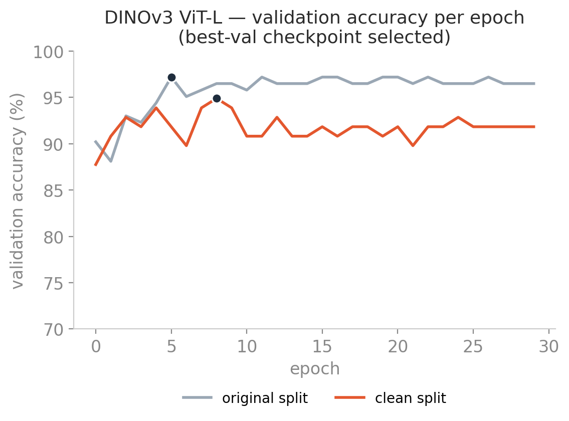
We train for 30 epochs but keep the best-validation checkpoint, not the last. The curve below shows why: clean-split accuracy peaks at epoch 8 (94.9%) and then drifts down as the small training set begins to overfit. Every number reported on this page is that peak checkpoint, and the prediction files used for the metrics come from it.
| Fine-tuning | Setting |
|---|---|
| Strategy | Frozen backbone + LoRA + new linear head |
| Trainable weights | LoRA (q_proj, v_proj) + head — ~3 MB |
| LoRA config | rank r=8 · α=16 · dropout 0.05 |
| Optimizer | AdamW · weight decay 0.05 |
| Learning rate | 1e-3 · cosine annealing |
| Epochs / batch | 30 / 16 · best-val checkpoint kept |
| Precision | AMP fp16 |
| Augmentation (online) | TrivialAugment + RandomErasing + MixUp/CutMix + label smoothing |
| Augmentation (corpus) | DiffuseMix (CVPR 2024) — clean training set expanded ~5× (395 → 1,975 generated views) |
| Hardware | single RTX 3060 (12 GB) |
| Seed | 42 |
Two splits, because the data leaks
Before trusting any accuracy number we checked the dataset itself. A perceptual-hash audit compared every image to every other and found 82 train↔val duplicate pairs — roughly half of the validation set are near-identical copies of training images. The models had effectively already seen part of the test set, so every number on the official split is optimistic. This is a normal data-quality issue in scraped datasets, not anyone's mistake.
So we built a leakage-proof split by construction: de-duplicate within each class (union-find over the perceptual hashes, keep the highest-resolution copy), then re-split 80/20 stratified with a fixed seed. 221 of 714 images — nearly 1 in 3 — were duplicates, leaving 493 unique images (395 train / 98 val). The originals are untouched and every change is logged. From here, accuracy means performance on genuinely unseen weapons.
The full leakage audit and de-duplication figures are on the case-study overview. Every metric below is reported on both splits so the inflation is visible.
Every metric, both splits
The deck shows one accuracy number; here is the full picture. Each metric appears on the leaky original split (n=143) and on the clean, leakage-proof split (n=98). Values are computed from the saved best-checkpoint predictions: precision/recall/F1 are macro-averaged over the nine classes, ROC-AUC and specificity are one-vs-rest then averaged, and MCC is the multiclass Matthews coefficient.
| Metric | Original (leaky) | Clean (honest) |
|---|---|---|
| Accuracy | 97.2% (139/143) | 94.9% (93/98) |
| Macro F1 | 0.973 | 0.948 |
| Weighted F1 | 0.972 | 0.949 |
| Macro precision | 0.974 | 0.953 |
| Macro recall | 0.974 | 0.949 |
| Macro ROC-AUC | 0.9995 | 0.9855 |
| MCC (multiclass) | 0.969 | 0.943 |
| Macro specificity | 0.997 | 0.994 |
Per-class precision, recall and F1 on bothsplits — the macro figures above are the unweighted mean of each table's rows. Every miss sits in the long-gun group; blades and the handgun are perfect on both.
Original (leaky) split · n=143
| Class | Precision | Recall | F1 | Support |
|---|---|---|---|---|
| Bazooka | 1.00 | 1.00 | 1.00 | 13 |
| Grenade launcher | 1.00 | 0.89 | 0.94 | 18 |
| Handgun | 1.00 | 1.00 | 1.00 | 14 |
| Knife | 1.00 | 1.00 | 1.00 | 14 |
| Rifle | 0.82 | 0.93 | 0.88 | 15 |
| Shotgun | 1.00 | 1.00 | 1.00 | 16 |
| SMG | 0.94 | 1.00 | 0.97 | 17 |
| Sniper | 1.00 | 0.94 | 0.97 | 18 |
| Sword | 1.00 | 1.00 | 1.00 | 18 |
Clean (leakage-proof) split · n=98
| Class | Precision | Recall | F1 | Support |
|---|---|---|---|---|
| Bazooka | 0.82 | 1.00 | 0.90 | 9 |
| Grenade launcher | 0.90 | 0.82 | 0.86 | 11 |
| Handgun | 1.00 | 1.00 | 1.00 | 11 |
| Knife | 1.00 | 1.00 | 1.00 | 10 |
| Rifle | 1.00 | 0.82 | 0.90 | 11 |
| Shotgun | 1.00 | 0.91 | 0.95 | 11 |
| SMG | 0.86 | 1.00 | 0.92 | 12 |
| Sniper | 1.00 | 1.00 | 1.00 | 11 |
| Sword | 1.00 | 1.00 | 1.00 | 12 |
Mistakes cluster among look-alike weapons
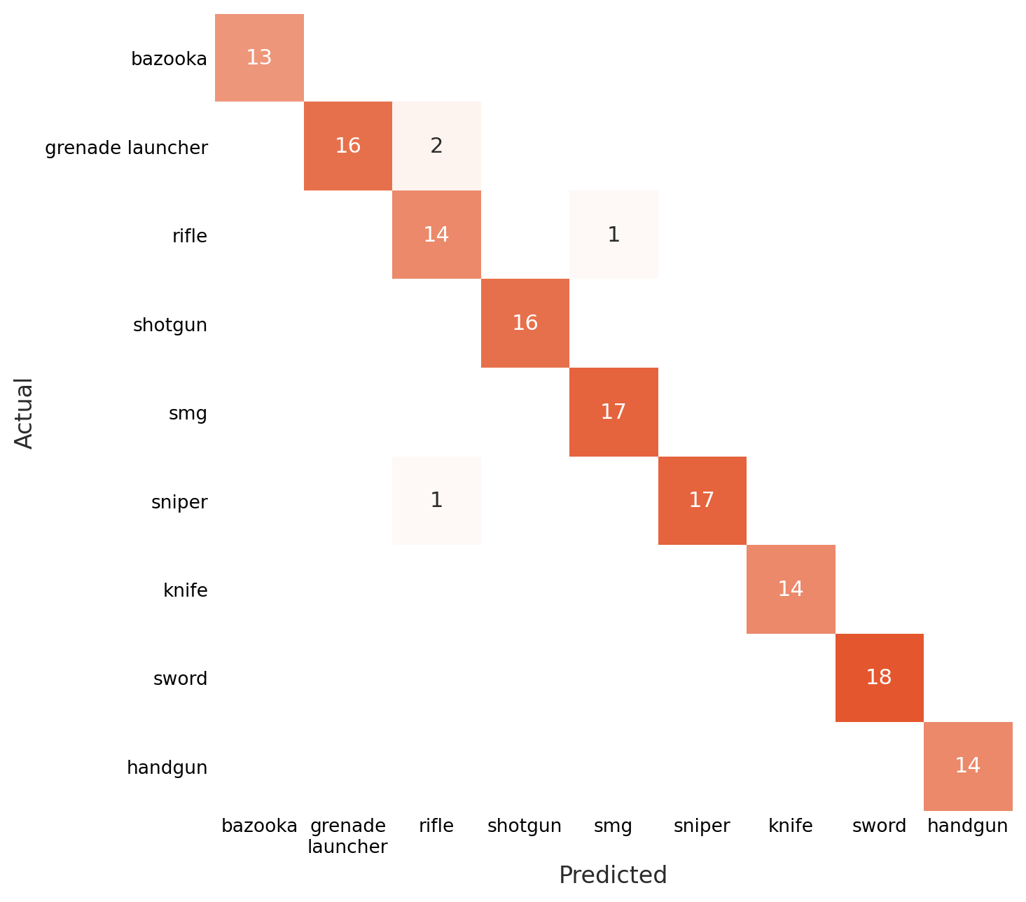
On the clean split DINOv3 misses 5 of 98 images, and every one is a long gun mistaken for another long gun — two grenade launchers, two rifles, one shotgun. The blades and the handgun are perfect.
The leakage gap collapses — and the frontier pair ties
Orange (Inception + LogReg)
−12.3 pts
DINOv3 ViT-L
−2.3 pts
ConvNeXt-V2-L
−-0.4 pts
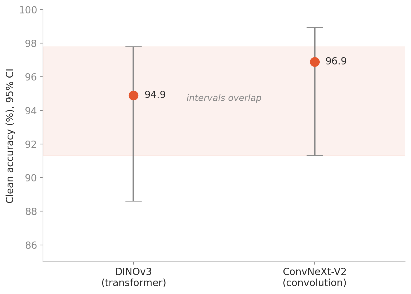
Stack the models weak-to-strong and the leakage gap collapses: the weak Inception+LogReg baseline drops ~12 points from the leaky to the clean split, while the two frontier models barely move. On the clean split DINOv3 and ConvNeXt — attention versus convolution — disagree on just 2 of 98 images. McNemar's exact test gives p = 0.50: the difference is not significant. They are tied, not ranked. When two opposite designs land in the same place, the dataset, not the model, is the ceiling.
| McNemar paired test | Original (leaky) | Clean (honest) |
|---|---|---|
| Discordant pairs (vs. the other frontier model) | 5 | 2 |
| Exact p-value | 1.00 | 0.50 |
Shown a non-weapon, it still picks a weapon
These are closed-set models: shown any image they must pick one of the nine weapon classes, even when there is no weapon in frame. We tested 27 everyday objects — cows, planes, vintage cars — and the classifier labelled every single one as a weapon. Its most confident mistake was a purple-painted cow called a "sword" at 85%.
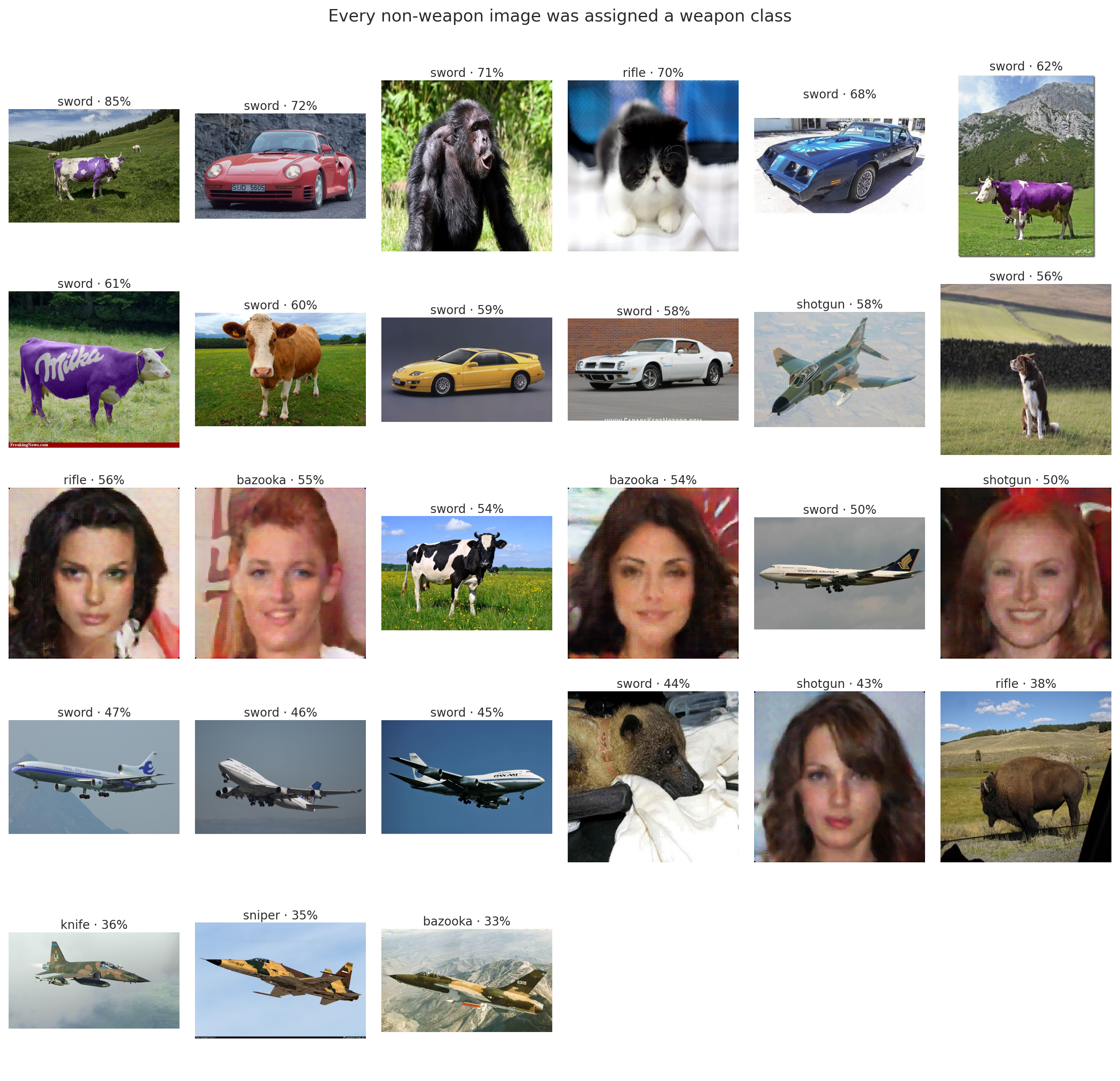
There is a signal to lean on: on real weapons confidence sits around 96%, on the non-weapons it falls to a median of ~55%. A confidence threshold near 0.80 would reject 26 of the 27 non-weapons — a good first defence, not a solution (the purple cow still sails through). The proper fix is an explicit "no weapon" class, and for real security use you would tune the threshold toward catching every real weapon.
Compare the other design
ConvNeXt-V2-L — Convolution · Modern CNN
Sources & further reading
A 9-class weapons image classifier, audited end to end: a dataset that leaks ~31% duplicates, the accuracy inflation that leakage hides, and two opposite frontier architectures that finish in a statistical tie on genuinely unseen images.